记忆网络(Memory network)
虚拟助理在回答单个问句时表现不赖,但是在多轮对话中表现差强人意,以下例子说明我们面临着什么挑战:
- Me: Can you find me some restaurants?
- Assistance: I find a few places within 0.25 mile. The first one is Caffé Opera on Lincoln Street. The second one is …
- Me: Can you make a reservation at the first restaurant?
- Assistance: Ok. Let’s make a reservation for the Sushi Tom restaurant on the First Street.
为什么虚拟助理不能按照我的指令预订Caffé Opera?那是因为虚拟助理并不能记住我们的对话,她只是简单地回答我们的问题而不考虑向前谈话的上下午。因此,她所能做的只是找到与词“First”相关的餐厅(一间位于First Street的餐厅)。记忆网络(Memory Networks)通过记住处理过的信息来解决该问题。
The description on the memory networks (MemNN) is based on Memory networks, Jason Weston etc.
考虑以下语句和问句“Where is the milk now?”:
- Joe went to the kitchen.
- Fred went to the kitchen.
- Joe picked up the milk.
- Joe traveled to the office.
- Joe left the milk.
- Joe went to the bathroom.
存信息于记忆
首先,保存句子在记忆m中:
| Memory slot \(m_i\) | Sentence |
|---|---|
| 1 | Joe went to the kitchen. |
| 2 | Fred went to the kitchen. |
| 3 | Joe picked up the milk. |
| 4 | Joe traveled to the office. |
| 5 | Joe left the milk. |
| 6 | Joe went to the bathroom. |
回答问句(Answering a query)
回答一个问句\(q\),首先通过打分函数\(s_0\)计算出与\(q\)最相关的句子\(m_{01}\)。然后将句子\(m_{01}\)与\(q\)结合起来形成新的问句\([q, m_{01}]\),并且定位最高分的下一个句子\(m_{01}\)。最后形成另外一个问句\([q, m_{01}, m_{02}]\)。此时我们并不是用该问句去查询下一个句,而是通过另一个打分函数定位一个词\(w\)。以上述例子来说明该过程。
回答问句\(q\)“where is the milk now?”,我们基于以下式子计算第一个推断:$$o_1 = \mathop{\arg\min}_{i=1,...,N}s_0(q, m_i)$$其中,\(s_0\)是计算输入\(x\)与\(m_i\)匹配分数的函数,\(o_1\)是记忆\(m\)中最佳匹配索引。这里\(m_{01}\)是第一个推断中最好的匹配句:“Joe left the milk.”。
然后,基于\([q: "where is the milk now", m_{01}: "Joe left the milk."]\)$$o_2
= \mathop{\arg\max}_{i=1,...,N}s_0([q, m_{01}], m_i)$$其中\(m_{02}\)是“Joe traveled to the office.”。
结合问句和推导的结果记为\(o\):$$o = [q, m_{01}, m_{02}] = ["where is the milk now"," Joe left the milk."," Joe travelled to the office."]$$生成最终的答复\(r\):$$r = \mathop{\arg\max}_{w \in W}s_r([q, m_{01}, m_{02}], w)$$其中\(W\)是字典中的所有词,\(s_r\)是另外一个计算\([q, m_{01}, m_{02}]\)和词\(w\)的匹配度。在我们的例子中,最后的回答\(r\)是“office”。
编码输入(Encoding the input)
我们利用词袋法(bags of words)表示输入文本。首先,我们以大小为\(\left|W\right|\)开始。
用词袋法对问句“where is the milk now”编码:
| Vocaulary | ... | is | Joe | left | milk | now | office | the | to | travelled | where | ... |
|---|---|---|---|---|---|---|---|---|---|---|---|---|
| where is the milk now | ... | 1 | 0 | 0 | 1 | 1 | 0 | 1 | 0 | 0 | 1 | ... |
"where is the milk now"=(...,1,0,0,1,1,0,1,0,0,1,...)
为了达到更好的效果,我们分别用三个词集编码\(q\),\(m_{01}\)和\(m_{02}\),即\(q\)中的词“Joe”编码为“Joe_1”,\(m_{01}\)中同样的词编码为“Joe_2”:
\(q\): Where is the milk now?
\(m_{01}\): Joe left the milk.
\(m_{02}\): Joe travelled to the office.
编码上述\(q, m_{01}, m_{02}\):
| ... | Joe_1 | milk_1 | ... | Joe_2 | milk_2 | ... | Joe_3 | milk_3 | ... |
|---|---|---|---|---|---|---|---|---|---|
| 0 | 1 | 1 | 1 | 1 | 0 |
因此,每一句变换为大小为\(3\left|W\right|\)的编码。
计算打分函数(Compute the scoring function)
我们用词嵌入\(U\)转换\(3\left|W\right|\)词袋编码的句子为大小为\(n\)的词嵌入表示。计算打分函数\(s_0\)和\(s_r\):$$s_0(x, y)n = \Phi_x(x)^TU_0^TU_0\Phi_y(y)$$ $$s_r(x, y)n = \Phi_x(x)^TU_r^TU_r\Phi_y(y)$$其中\(U_0\)和\(U_r\)由边缘损失函数训练得到,\(\phi(m_i)\)转换句子\(m_i\)为词袋表示。
边缘损失函数(Margin loss function)
用边缘损失函数训练\(U_0\)和\(U_r\)中的参数:
$$\sum\limits_{\overline{f}\not=m_{01}}\max(0, \gamma - s_0(x, m_{01}) + s_0(x, \overline{f})) + $$ $$\sum\limits_{\overline{f}\not=m_{02}}\max(0, \gamma - s_0(\left[x, m_{01}\right], m_{02}) + s_0(\left[x, m_{01}\right], \overline{f^\prime})) + $$ $$\sum\limits_{\overline{r}\not=r}\max(0, \gamma - s_0(\left[x, m_{01}, m_{02}\right], r) + s_0(\left[x, m_{01}, m_{02}\right], \overline{r}))$$其中\(\overline{f}\),\(\overline{f^\prime}\)和\(\overline{r}\)是真实标签外的其它可能预测值。即当错误回答的分数大于正确回答的分数减\(\gamma\)时增加边缘损失。
大记忆网络(Huge memory networks)
对于记忆规模较大的的系统,计算每个记忆的分数较昂贵。其它可选方案为,计算完词嵌入\(U_0\)后,运用K-clustering将词嵌入空间分为K类。然后将每个输入\(x\)映射到相应类中,并在类空间中进行推测而不是在全部记忆空间中。
端到端记忆网络(End to End memory network, MemN2N)
The description, as well as the diagrams, on the end to end memory networks (MemN2N) are based on End-To-End Memory Networks, Sainbayar Sukhbaatar etc..
以一句问句“where is the milk now?”开始,并用大小为\(V\)的词袋表示(其中\(V\)为词典大小)。简单地,用词嵌入矩阵\(B(d\times V)\)转换上述向量为\(d\)维词嵌入。$$u = embedding_B(q)$$ 对于每个记忆项\(x_i\),用另一个词嵌入矩阵\(A(d\times V)\)转换为d维向量\(m_i\)。$$m_i = embedding_A(x_i)$$
通过计算\(u\)与每个记忆\(m_i\)的内积然后softmax得到其匹配度:$$p_i =
softmax(u^Tm_i)$$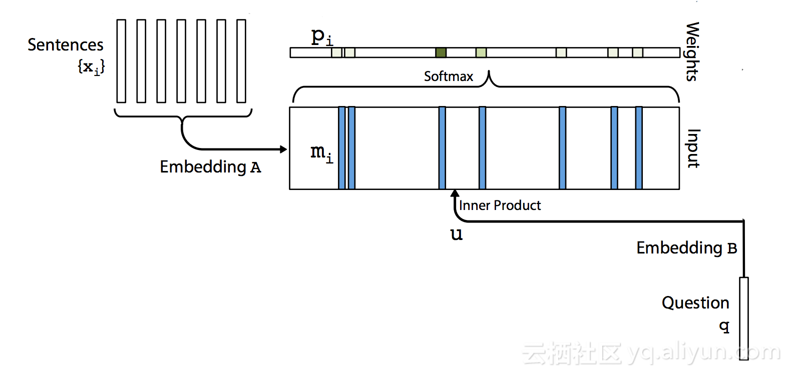
用第三个词嵌入矩阵编码\(x_i\)为\(c_i\):$$c_i = emedding_C(x_i)$$ 计算输出:$$o = \sum\limits_{i}p_ic_i$$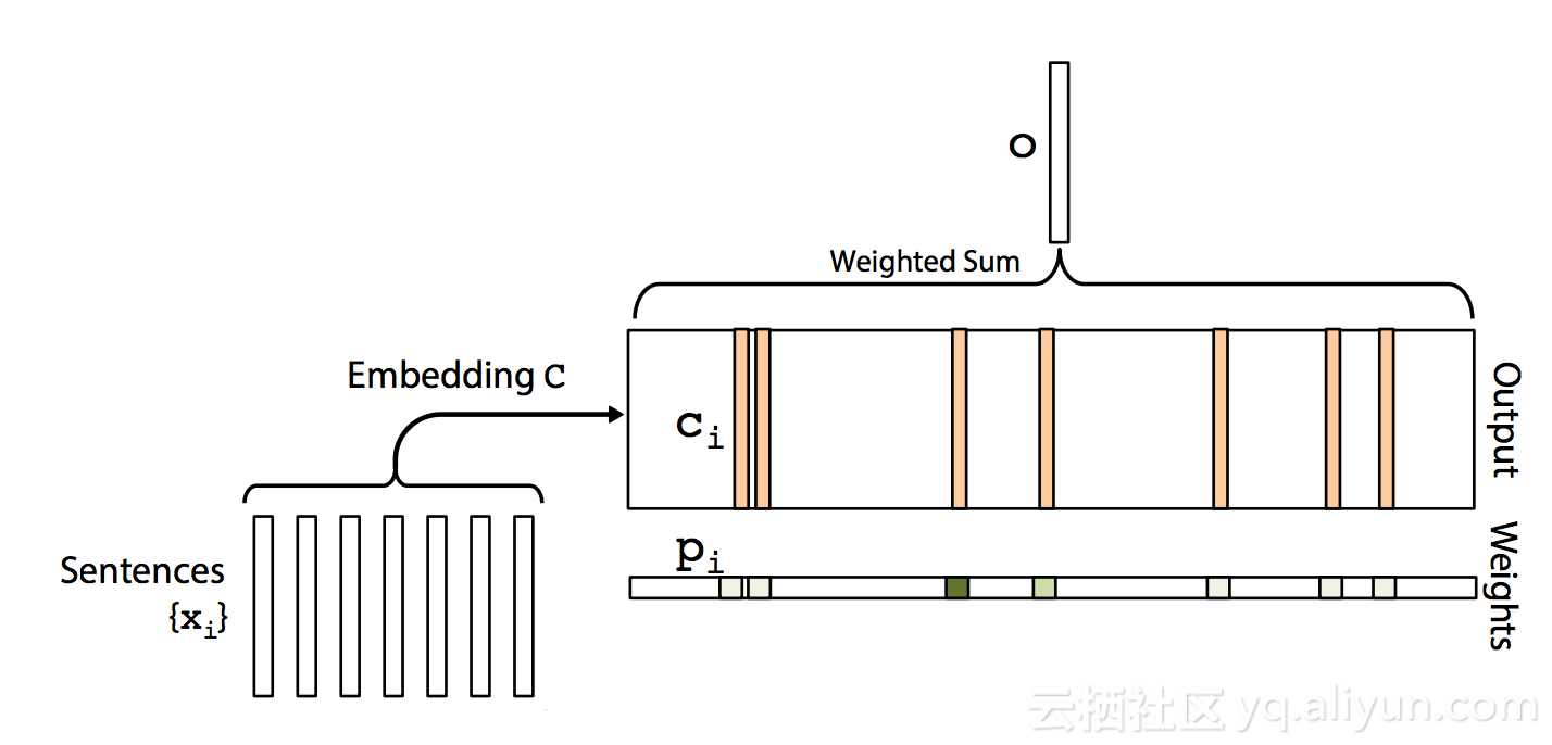
用矩阵\(W(V\times d)\)乘以\(o\)和\(u\)的和。结果传给softmax函数预测最终答案。$$\hat a = softmax(W(o + u))$$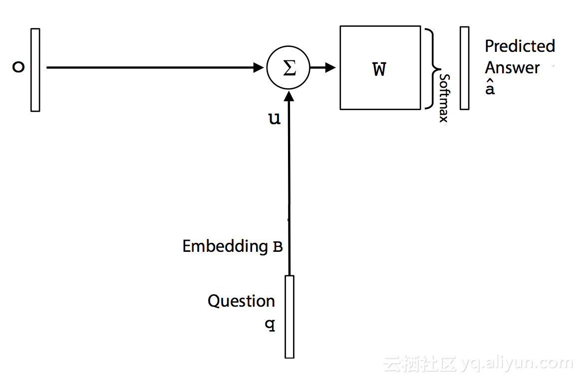
这里,将所有步骤总结为一个图: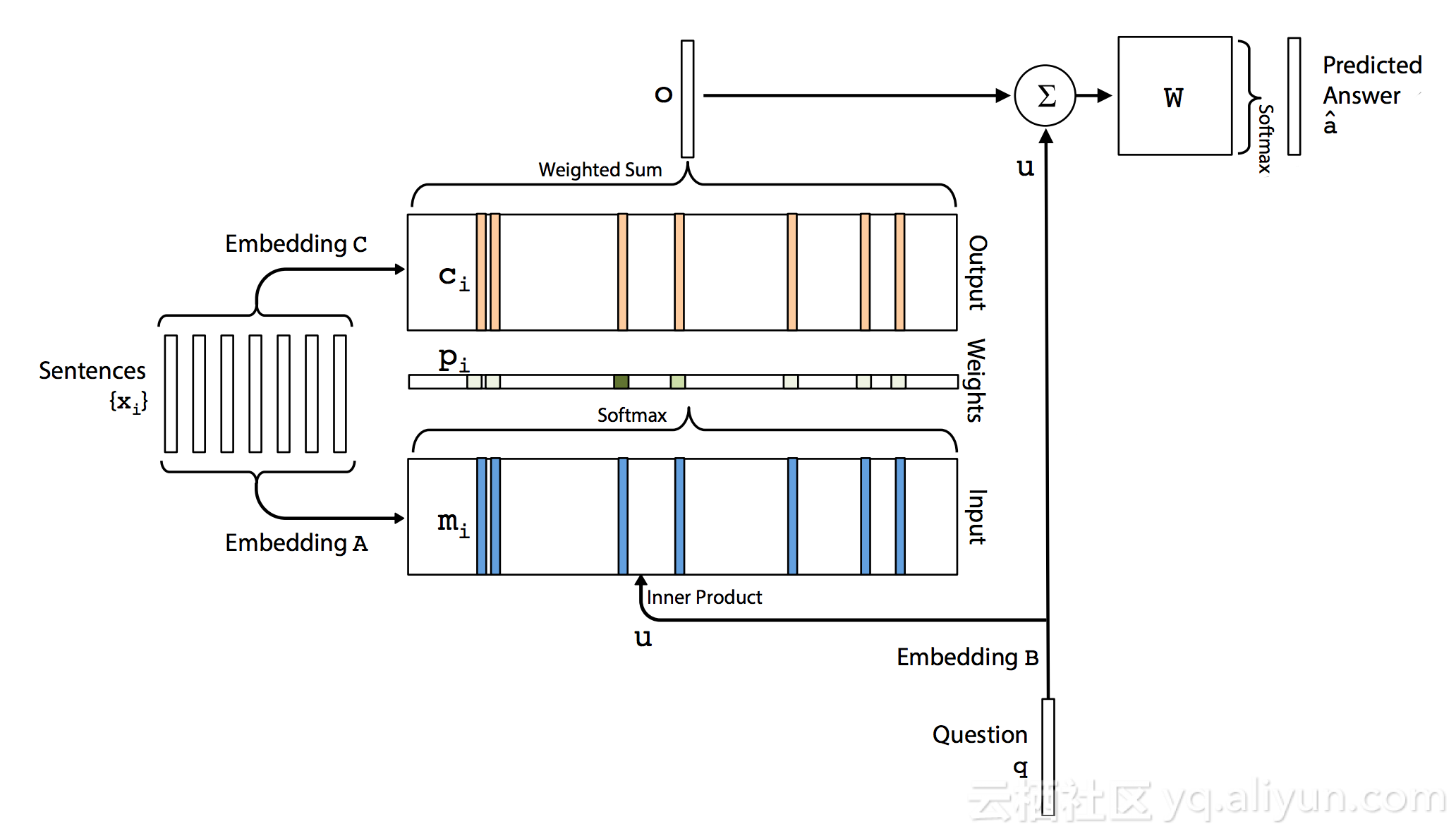
多层(Multiple layer)
与RNN类似,可以堆叠多层形成复杂网络。在每一层\(i\),有它自己的嵌入矩阵\(A_i\)和\(C_i\)。层\(k + 1\)的输入为:$$u^{k + 1} = u^k + o^k$$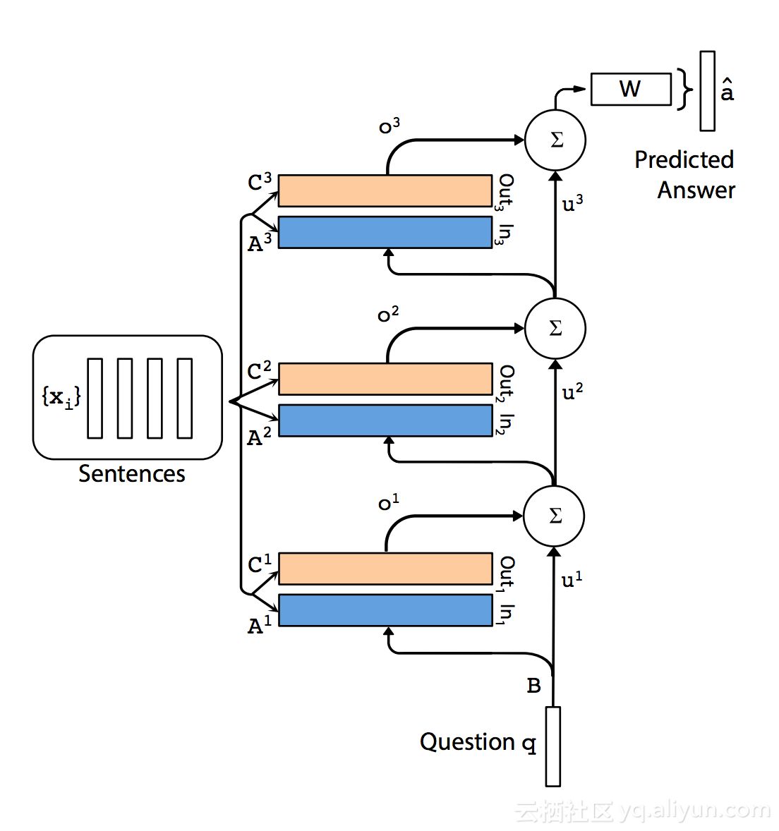
语言模型(Language model)
可以用MemN2N作为语言模型。比如,解析“独立申明”:“We hold these truths to be self-evident, that all men are created equal, that they are endowed by their Creator with certain unalienable Rights, that among these are Life, Liberty and the pursuit of Happiness.”,不是每一句为一个记忆项而是没一词为一项:
| Memory slot \(m_i\) | word |
|---|---|
| 1 | We |
| 2 | hold |
| 3 | these |
| 4 | truths |
| 5 | to |
| 6 | be |
| 7 | ... |
上述语言模型的目的是预测第7个词。
根据MemN2N论文中的描述,其不同有:
1. 没有问句,我们试着找下个词而不是问句的答案。因此,我们无需词嵌入矩阵B,只需以常量0.1填充\(u\)。
2. 我们使用多层,但是每层词嵌入矩阵\(A\)相同,而词嵌入矩阵\(B\)不同。
3. 词嵌入增加时间项来记录记忆中词的次序(Section 4.1)。
4. 加上\(o\)前,使\(u\)乘以一个线性向量。
5. 为了帮助训练,对每层的一半单元运用ReLU(Section 5)。
以下是构建嵌入\(A\),\(C\),\(m_i\),\(c_i\),\(p\),\(o\)和\(\hat a\)的代码。
def build_memory(self):
    self.A = tf.Variable(tf.random_normal([self.nwords, self.edim], stddev=self.init_std)) # Embedding A for sentences
    self.C = tf.Variable(tf.random_normal([self.nwords, self.edim], stddev=self.init_std)) # Embedding C for sentences
    self.H = tf.Variable(tf.random_normal([self.edim, self.edim], stddev=self.init_std))   # Multiple it with u before adding to o

    # Sec 4.1: Temporal Encoding to capture the time order of the sentences.
    self.T_A = tf.Variable(tf.random_normal([self.mem_size, self.edim], stddev=self.init_std))
    self.T_C = tf.Variable(tf.random_normal([self.mem_size, self.edim], stddev=self.init_std))

    # Sec 2: We are using layer-wise (RNN-like) which the embeddings for each layers are sharing the parameters.
    # (N, 100, 150) m_i = sum A_ij * x_ij + T_A_i
    m_a = tf.nn.embedding_lookup(self.A, self.sentences)
    m_t = tf.nn.embedding_lookup(self.T_A, self.T)
    m = tf.add(m_a, m_t)

    # (N, 100, 150) c_i = sum C_ij * x_ij + T_C_i
    c_a = tf.nn.embedding_lookup(self.C, self.sentences)
    c_t = tf.nn.embedding_lookup(self.T_C, self.T)
    c = tf.add(c_a, c_t)

    # For each layer
    for h in range(self.nhop):
        u = tf.reshape(self.u_s[-1], [-1, 1, self.edim])
        scores = tf.matmul(u, m, adjoint_b=True)
        scores = tf.reshape(scores, [-1, self.mem_size])

        P = tf.nn.softmax(scores)     # (N, 100)
        P = tf.reshape(P, [-1, 1, self.mem_size])

        o = tf.matmul(P, c)
        o = tf.reshape(o, [-1, self.edim])

        # Section 2: We are using layer-wise (RNN-like), so we multiple u with H.
        uh = tf.matmul(self.u_s[-1], self.H)
        next_u = tf.add(uh, o)

        # Section 5:  To aid training, we apply ReLU operations to half of the units in each layer.
        F = tf.slice(next_u, [0, 0], [self.batch_size, self.lindim])
        G = tf.slice(next_u, [0, self.lindim], [self.batch_size, self.edim-self.lindim])
        K = tf.nn.relu(G)
        self.u_s.append(tf.concat(axis=1, values=[F, K]))

    self.W = tf.Variable(tf.random_normal([self.edim, self.nwords], stddev=self.init_std))
    z = tf.matmul(self.u_s[-1], self.W)
计算损失,通过梯度修剪构建优化器
self.loss = tf.nn.softmax_cross_entropy_with_logits(logits=z, labels=self.target)

self.lr = tf.Variable(self.current_lr)
self.opt = tf.train.GradientDescentOptimizer(self.lr)

params = [self.A, self.C, self.H, self.T_A, self.T_C, self.W]
grads_and_vars = self.opt.compute_gradients(self.loss, params)
clipped_grads_and_vars = [(tf.clip_by_norm(gv[0], self.max_grad_norm), gv[1]) \
                                   for gv in grads_and_vars]

inc = self.global_step.assign_add(1)
with tf.control_dependencies([inc]):
      self.optim = self.opt.apply_gradients(clipped_grads_and_vars)
训练
def train(self, data):
    n_batch = int(math.ceil(len(data) / self.batch_size))
    cost = 0

    u = np.ndarray([self.batch_size, self.edim], dtype=np.float32)      # (N, 150) Will fill with 0.1
    T = np.ndarray([self.batch_size, self.mem_size], dtype=np.int32)    # (N, 100) Will fill with 0..99
    target = np.zeros([self.batch_size, self.nwords])                   # one-hot-encoded
    sentences = np.ndarray([self.batch_size, self.mem_size])

    u.fill(self.init_u)   # (N, 150) Fill with 0.1 since we do not need query in the language model.
    for t in range(self.mem_size):   # (N, 100) 100 memory cell with 0 to 99 time sequence.
       T[:,t].fill(t)

    for idx in range(n_batch):
        target.fill(0)      # (128, 10,000)
        for b in range(self.batch_size):
            # We random pick a word in our data and use that as the word we need to predict using the language model.
            m = random.randrange(self.mem_size, len(data))
            target[b][data[m]] = 1                       # Set the one hot vector for the target word to 1

            # (N, 100). Say we pick word 1000, we then fill the memory using words 1000-150 ... 999
            # We fill Xi (sentence) with 1 single word according to the word order in data.
           sentences[b] = data[m - self.mem_size:m]

            _, loss, self.step = self.sess.run([self.optim,
                                                self.loss,
                                                self.global_step],
                                                feed_dict={
                                                    self.u: u,
                                                    self.T: T,
                                                    self.target: target,
                                                    self.sentences: sentences})
            cost += np.sum(loss)

    return cost/n_batch/self.batch_size
初始化
class MemN2N(object):
    def __init__(self, config, sess):
        self.nwords = config.nwords         # 10,000
        self.init_u = config.init_u         # 0.1 (We don't need a query in language model. So set u to be 0.1
        self.init_std = config.init_std     # 0.05
        self.batch_size = config.batch_size # 128
        self.nepoch = config.nepoch         # 100
        self.nhop = config.nhop             # 6
        self.edim = config.edim             # 150
        self.mem_size = config.mem_size     # 100
        self.lindim = config.lindim         # 75
        self.max_grad_norm = config.max_grad_norm   # 50

        self.show = config.show
        self.is_test = config.is_test
        self.checkpoint_dir = config.checkpoint_dir

        if not os.path.isdir(self.checkpoint_dir):
            raise Exception(" [!] Directory %s not found" % self.checkpoint_dir)

        # (?, 150) Unlike Q&A, the language model do not need a query (or care what is its value).
        # So we bypass q and fill u directly with 0.1 later.
        self.u = tf.placeholder(tf.float32, [None, self.edim], name="u")

        # (?, 100) Sec. 4.1, we add temporal encoding to capture the time sequence of the memory Xi.
        self.T = tf.placeholder(tf.int32, [None, self.mem_size], name="T")

        # (N, 10000) The answer word we want. (Next word for the language model)
        self.target = tf.placeholder(tf.float32, [self.batch_size, self.nwords], name="target")

        # (N, 100) The memory Xi. For each sentence here, it contains 1 single word only.
        self.sentences = tf.placeholder(tf.int32, [self.batch_size, self.mem_size], name="sentences")

        # Store the value of u at each layer
        self.u_s = []
        self.u_s.append(self.u)
完整代码在github
动态记忆网络(Dynamic memory network)
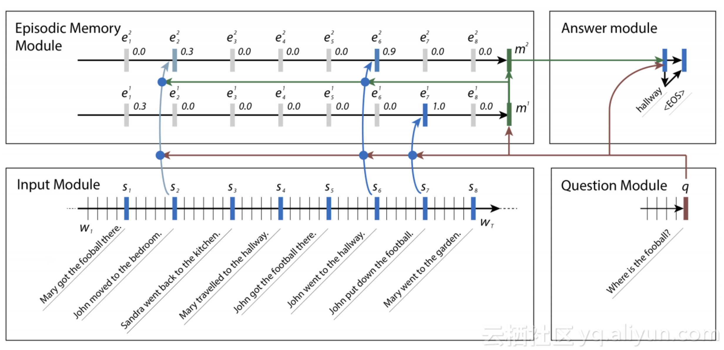
Sentence
句子由GRU处理,其中最后隐藏状态用于记忆模块。